Image enhancement, or image quality improvement is one of the early processes in image processing. Improved image quality is required because often the image being made object have the quality not match as expected. The histogram in the grayscale image represents the distribution of the gray degree in an image. From this histogram can be seen whether the image is more dark color or more bright colors. Look at the picture below.
 |
| Figure 1. An example of a grayscale image |
Figure 1 is actually a color image. But in this lab all colored images will be grayscale images. Figure 1 certainly has its own histogram value. Here is the histogram value of Figure 1.
 |
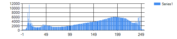
| Figure 2. Histogram in Figure 1 |
Figure 2 is a histogram of Figure 1. If the value is seen in the graph, the value distribution is at most between the 30 to 99, so it has a dark dominant color. If you look again, the value above 149 is lower than the value below 149. It can be seen in Figure 1 is more dominant dark color than the light color.
So what if Image 1 is subject to one of the image enhancement process, ie inverse. Here is the result.
 |
| Figure 3. The inverse results from Figure 1 |
In contrast to Fig. 1, in Fig. 3 the entire black-and-white component of Fig. 1 is reversed. Color pixels that had been valuable eg 90, to be worth 165. Color pixel that was dominant dark, became dominant light. Vice versa. Then what is the impact of the inverse on the resulting histogram? Have a look at the picture below.
 |
| Figure 4. Results of histogram in Figure 3 |
The histogram in Figure 4 has a difference in the histogram in Figure 2. Figure 4 has a value that is inversely proportional to the value in Fig.2. This is due to the inverse occurring in Fig. What if the image is exposed to the brightness effect? Look at the image below.
 |
| Figure 5. The effect of brightness with the addition of +10 |
Figure 5 is Figure 1 are affected by the addition of +10 brightness value. It looks much brighter when compared to Figure 1. That is because each color value in Figure 1 is added to a constant value, in this case the constants are +10. So the colors close to white and produce bright colors.
Then what about the histogram value? Notice the chart below.
 |
| Figure 6. Histogram value for brightness with value of +10 addition |
It can be seen in Figure 6 that the histogram value shifts to the right, in other words it shifts to 255. That is because in the brightness effect the original color will be added by the constant, in this case the constant is +10. So the color values will converge to 255 points. For more details please see the histogram changes for the brightness effect with the constants +10, +11, and +12 below.
 |
| Figure 7. Histogram values for brightness effects with constants +10, +11, and +12 |
Although less obvious because of scale constraints, but in Figure 7 clearly displays the value of the histogram from left to right. For more details can be seen the number of values 255 on each histogram. The greater the addition of the brightness value, the greater the value of 255. So what if the brightness constant is negative? Look at the image below.
 |
| Figure 8. The effect of brightness with a value of -10 |
Figure 8 is Figure 1 are exposed to the effects of the addition of -10 brightness value. It looks much darker when compared to Figure 1. That is because each color value in Figure 1 is added to a constant value, in this case the constant is -10. So that the color close to black and produce a dark color. Then what about the histogram value? Notice the chart below.
 |
| Figure 9. The histogram value for brightness with a -10 increment value |
It can be seen in Figure 9 that the histogram value shifts to the left, in other words it shifts to a value of 0. This is because in effect the brightness of the original color will be added by the constant, in this case the constant is -10. So the color values will converge to the point 0. For more details please see the histogram changes for the brightness effect with the -10, -11, and -12 constants below.
 |
| Figure 10. Histogram values for brightness effects with constants -10, -11, and -12 |
Although less obvious because of scale constraints, but in Figure 10 it is clear to shift histogram value from right to left. For more details can be seen the number of values 0 on each histogram. The smaller the addition of the brightness value, the greater the value of 0. Contrast is the process of raising the difference of light and dark values of an image by multiplying the value of gray degree with the value of contrast change. Look at the image below.
 |
| Figure 11. Contrast effect with constant value 1.1 |
Figure 11 is Figure 1 are exposed to the effects of contrast with the constant value of 1.1. It looks much brighter when compared to Figure 1. Unlike the brightness, the contrast effect results in a light-dark change of the image at certain points only, not spreading like brightness. Note the value of the resulting histogram.
 |
| Figure 12. Histogram value for contrast with constant value 1.1 |
Unlike the brightness, the contrast has a very significant change. If the value of constant is more than 1, then the addition will be more to 255, or the value with white. So what if the contrast constant is less than 1? Look at the image below.
 |
| Figure 12. Contrast effect with constant value 0.9 |
Figure 12 is Figure 1 are exposed to the effects of contrast with the constant value of 0.9. It looks much darker when compared to Figure 1. Then what about the histogram value? Note the value of the resulting histogram.
 |
| Figure 13. Histogram value for contrast with constant value 0.9 |
It appears that there is a change only in certain points of value. The histogram value still has not converged in value 0 because the image is still relatively bright. If the value of a constant is between 0 and 1, then the addition will be more to the value 0, or the value with black. For a detailed discussion of the histogram, note the image below.
 |
| Figure 14. Image with bright dominant |
One of the purposes of the histogram is to see if an image has more light or dark colors. If seen in Figure 14, the distribution of histogram values will be more on the right. Here is a picture of his histogram.
 |
| Figure 15. The histogram graph of Figure 14 |
The graph on the right in Figure 15 is more because Figure 14 is dominated by light colors. Bright colors have a color range between 128 and 255. So among the range that will have many values.
Look at the image below.
 |
| Figure 16. Image with dark dominant |
When viewed in Figure 16, the distribution of histogram values will be more on the left. Here is a picture of his histogram.
 |
| Figure 17. The histogram graph in Figure 16 |
The graph on the left of Figure 17 is more because Figure 16 is dominated by dark colors. Dark colors have a color range between 0 to 128. So among the range that will have many values. The cumulative distribution is the total value of the histogram from the gray level 0 to the gray level x. This cumulative distribution can be used to show the color progression of each gray step step. In the cumulative distribution, the image is well represented if it has a nearly equal distribution of movement at all degrees of gray. Look at the image below.
 |
| Figure 18. Sample image for cumulative distribution |
Figure 18 has a color change that is too sharp, from dark directly to white. This shows the level of gradation on the image is low (rough). Here is the resulting cumulative or CDF distribution.
 |
| Figure 19. Cumulative distribution in Figure 18 |
Seen in Figure 19 has a sharp change. This is because the image used has a low gradation level or rough. So that impact on the resulting CDF. Look at the image below.
 |
| Figure 20. Sample image for cumulative distribution |
Figure 20 has a non-sharp color change. This shows the level of gradation on the high image (smooth). Here is the resulting cumulative or CDF distribution.
 |
| Figure 21. Cumulative distribution in Figure 20 |
Seen in Figure 21 has a subtle change. This is because the image used has a high level of gradation. So that impact on the resulting CDF. In the histogram there is also a PDF term, or Probability Density Function. PDF is a group of functions that are often used in statistical theory to explain the perilau of a probability distribution, in this case is color. The colors on the image will be compared to the pixel area in the image. So the resulting value is in the range of 0 to 1. Look at the image below.
 |
| Figure 22. Sample image for PDF |
Then look at value of the histogram and PDF value below
 |
| Figure 23. The value of histogram and PDF in Figure 22. |
Seen in Figure 23 that the graphs generated by histogram and PDF are the same, only the values are different. Because the PDF states the color probability in all pixels of the image.
Go to to next part
Writer : hamuhamu & asrul

Comments
Post a Comment