This time we will try different types of filters for image processing. There are three filter principles in image processing, namely:
- Low Pass Filter (LPF) is used to remove a different point with its neighboring points, or in other words the noise reduction process. LPF will take data at low frequencies and discard data at high frequencies.
- High Pass Filter (HPF) is used to maintain a different point with its neighboring points, or in other words edge detection process. HPF will take data at high frequencies and dump data at low frequencies.
- Band Pass Filter (BPF) is used to maintain a point close to the neighboring points, and a point different from the neighboring points, in other words the sharperness process. BPF will maintain low and high frequencies that are not too low and high.
Low Pass Filter for noise reduction process
Based on the above three principles, LPF is used to reduce noise on the image. Noise itself has three types, namely gaussian noise, speckle noise, and salt and papper noise. For more details, please see below.
 |
| Figure 1. Original Graph with Gray Degrees for LPF Experiments |
Figure 1 is an original image that has been converted into an image with a gray degree. Then notice what happens if the image is added different types of noise.
 |
| Figure 2. (a) Gaussian Noise, (b) Speckle Noise, (c) Salt and Pepper Noise |
FIG. 2 is an example of the result of FIG. 1 which added some noise from three different noise types. In the noise gaussian, the emerging noise has a random color range of 0 to 255. It can be seen in figure (a) that still has the dominant color with its original color (not dominant black or white). In speckle noise, the noise that appears has a black or 0 color so that in the picture (b) has a black dominant color. While the salt and pepper noise, the noise that appears has a white color or 255 so that the picture (c) has a predominantly white color. After the image has noise, the noise can be reduced using LPF. There are three types of filters on the LPF that can be used to reduce noise. They are average filters, gaussian filters, and median filters. Keep using the same image, let's experiment with reducing noise in the image using three different types of LPF filters. We will generate three types of noise with probability values of 5%, 20%, 50%, 80%, and 95% noise occurrence.
Image with probability value of noise occurrence 5%
Here is the result of noise with probability value 5% :
 |
| Figure 3. (a) Gaussian Noise, (b) Speckle Noise, (c) Salt and Pepper Noise With Probability 5% |
Noise that appears on the image looks not too dominant because of the small probability value. Although not dominant, noise remains visible and noise reduction needs to be done. First, we will try to use the average filter. Here is the result of the reduction for each type of noise.
 |
| Figure 4. Noise Reduction Result Using Average Filter. (a) Gaussian Noise, (b) Speckle Noise, (c) Salt and Papper Noise With Probability Value 5% |
It can be seen in Figure 4 that the noise has decreased slightly although not seen significantly. This is because the probability value of the emergence of noise that only reaches 5% so it is still difficult to distinguish the image that has not been reduced. Secondly, we will try to reduce the noise using gaussian filter. Here is the result.
 |
| Figure 5. Noise Reduction Result Using Gaussian Filter. (a) Gaussian Noise, (b) Speckle Noise, (c) Salt and Papper Noise With Probability Value 5% |
Figure 5 is the result of noise reduction using a gaussian filter. When viewed, the noise reduction result using a gaussian filter is almost the same as the average filter in Figure 4. This is because the kernel value of the matrices of both filters has an approximate value. Here is the matrix value for both filters.
 |
| Figure 6. Matrix Kernel Value (a) Average Filter and (b) Gaussian Filter |
The kernel value in the matrix in Figure 6 is fractionally different. However, if it is minimized, then the kernel value of the two matrices will have a value close to (less than 1). So the resulting image also has almost the same results. Despite that, the two noise reduction results are still different. It can be proven through the histogram value. Here is a histogram graph for both filters.
 |
| Figure 7. Histogram Graph (a) Average Filter and (b) Gaussian Filter |
Figure 7 is the histogram value for both filters on the gaussian noise. It is seen that both graphs have different histogram values which are located at their highest values. So the average filter and the gaussian filter have different histogram values even though the noisenya reduction results are almost identical. Finally, we will try to reduce the noise by using the median filter. Here is the result.
 |
| Figure 8. Noise Reduction Result Using Median Filter. (a) Gaussian Noise, (b) Speckle Noise, (c) Salt and Papper Noise With Probability Value 5% |
Figure 8 is the noise reduction result using a median filter. Theoretically, the median filter is the best filter when compared to the other two filters, and it can be proved by a smoother result. This is influenced by the median filter method which takes the middle value of all the color values from its sorted neighbor point. In addition, that affects the filter results are smoother because the probability value of the occurrence of noise is still small.
Image with probability value of noise occurrence 20%
In the previous experiment we have tried to use a probability value of 5%. Now what changes if we use a probability value of 20%? Here are the noisenya results.
 |
| Figure 9. (a) Gaussian Noise, (b) Speckle Noise, (c) Salt and Pepper Noise With Probability 20% |
Noise that appears in the image looks more dominant when compared with previous experiments. Noise is more clearly visible, especially in salt and papper noise. This is because the image has a dark dominant color while salt and papper noise produces noise with white. First, we will try to use the average filter. Here is the result of the reduction for each type of noise.
 |
| Figure 10. Noise Reduction Result Using Average Filter. (a) Gaussian Noise, (b) Speckle Noise, (c) Salt and Papper Noise With Probability Value 20% |
It can be seen in Figure 10 that the noise is still visible even though it has been reduced, even more so on the obvious salt and papper noise. This is because the probability value is already high although not yet reached the value of 50%. Secondly, we will try to reduce the noise using gaussian filter. Here is the result.
 |
| Figure 11. Noise Reduction Result Using Gaussian Filter. (a) Gaussian Noise, (b) Speckle Noise, (c) Salt and Papper Noise With Probability Value 20% |
Figure 11 is the result of noise reduction using a gaussian filter. Still has the same result as Figure 10, that noise still looks dominant in the picture. This is because the value of the relatively high probability of noise. Finally, we will try to reduce the noise by using the median filter. Here is the result.
 |
| Figure 12. Noise Reduction Result Using Median Filter. (a) Gaussian Noise, (b) Speckle Noise, (c) Salt and Papper Noise With Probability Value 20% |
Figure 12 is the noise reduction result using a median filter. It has been mentioned in the previous experiment that the median filter is the best filter for noise reduction and is shown in Figure 12. Notice in the salt and papper noise section, the noise can be reduced optimally which can not be done by the two previous filters, although there are still points remaining noise.
Image with probability value of noise occurrence 50%
In this experiment we will use a probability value of 50% noise emission. So the noise that comes later has a balanced comparison. Here are the noisenya results.
 |
| Figure 13. (a) Gaussian Noise, (b) Speckle Noise, (c) Salt and Pepper Noise With Probability 50% |
It can be seen in Figure 13 that the noise is increasing and covering the original image. This is because the probability value of the occurrence of noise is higher. First, we will try to use the average filter. Here is the result of the reduction for each type of noise.
 |
| Figure 14. Noise Reduction Result Using Average Filter. (a) Gaussian Noise, (b) Speckle Noise, (c) Salt and Papper Noise With Probability Value 50% |
It can be seen in Figure 14 that the noise is still visible even though it has been reduced, even more so on the obvious salt and papper noise. Secondly, we will try to reduce the noise using gaussian filter. Here is the result.
 |
| Figure 15. Noise Reduction Result Using Gaussian Filter. (a) Gaussian Noise, (b) Speckle Noise, (c) Salt and Papper Noise With Probability Value 50% |
Figure 15 is the result of noise reduction using a gaussian filter. Noise still looks dominant in the picture. This is because the value of the relatively high probability of noise. Finally, we will try to reduce the noise by using the median filter. Here is the result.
 |
| Figure 12. Noise Reduction Result Using Median Filter. (a) Gaussian Noise, (b) Speckle Noise, (c) Salt and Papper Noise With Probability Value 50% |
Seen in Figure 12 the noise is still visible, especially on the gaussian speckle noise and salt and papper noise. While on gaussian noise, noise is not so clearly visible. This is because the color of the noise is not fixated with black or white, so the color of the noise can be disguised.
High Pass Filter for edge detection process
HPF is the type of filter used to pass high frequencies. High frequency in terms of the high degree of color difference in imagery. So HPF used to detect the edge on the image. Edge detection is the process of getting edge information from an image. There are several methods commonly used to perform edge detection, namely prewitt method, sobel, and laplacian. For more details please see the experiment below.
 |
| Figure 13. Cartoon Image With Gray Degrees For HPF Experiments |
Figure 13 is an image sample to be used for the experiment. We use cartoon images because cartoon images have many high frequencies and minimal color gradations. So it will get optimal results when we do edge detection. Here are the results of edge detection using all three methods.
 |
| Figure 14. Edge Detection Results. (a) Prewitt method, (b) Sobel method, (c) Laplacian method |
It can be seen in Figure 14 that each method has different results. In the prewitt method, the resulting edge detection has a darker color when compared to the other two methods. In the sobel method, the resulting edge detection has the brightest color. In the visible also motedo sobel almost the same as the prewitt method. The laplacian method has a slightly less sharp edge detection result. Because the laplacian method only detects sharp edges only, so it has a low sensitivity level. On edge detection is also known as binaryization. For more details please see image below.
 |
| Figure 15. Binary Process In Edge Detection Results. (a) Prewitt method, (b) Sobel method, (c) Laplacian method |
Binary process is the process of changing the color of the image so it only has two colors only, that is black with color values 0 and white with 255 color values. Technically, the process done on binary is to check the entire pixel color. If the color value of a pixel is less than 128, then the color value of the pixel will be changed to 0. Whereas the color value in a pixel is more than equal to 128, then the color value will be changed to 255. Seen in Figure 15 after the result done binary process is the image becomes sharper because the remaining color is just black and white. In addition to binary, there is also an inverse term. Here is the result.
 |
| Figure 16. Inverse Process In Edge Detection Results. (a) Prewitt method, (b) Sobel method, (c) Laplacian method |
The inverse process will reverse the color values of each image pixel. The color that was originally dominant black will be the dominant white, and vice versa. In Figure 16, the result of edge detection will be more obvious and can prove that the sobel method has a sharper result when compared to the prewitt method. So what happens if binary and inverse are done simultaneously on the edge detection process? Here are the experimental results.
 |
| Figure 17. Binary and Inverse Process In Edge Detection Results. (a) Prewitt method, (b) Sobel method, (c) Laplacian method |
Merging the binary and inverse processes will produce a black-and-white image with a white background and black edges. In Figure 17 the image becomes sharper and the edges of the image become more visible because on the edge there is only black. After we try to use a cartoon image, this time we will experiment with normal images that have more color gradations. Here is the experiment.
 |
| Figure 18. Normal Picture With Gray Degrees For HPF Experiments |
Unlike the picture cards, Figure 18 has a lot of color tiitk with a considerable low frequency level. Later we can see how the three methods can select the point of color with high frequency and discard the color point with low frequency so that edge can be detected. Here are the results of edge detection using all three methods.
 |
| Figure 19. Edge Detection Results. (a) Prewitt method, (b) Sobel method, (c) Laplacian method |
It can be seen in Figure 19 that each method has different results. In the prewitt method, the resulting edge detection has a darker color when compared to the other two methods. In the sobel method, the resulting edge detection has the brightest color. In the visible also motedo sobel almost the same as the prewitt method. The result of laplacian method only produces dark black color because in the picture there is no very high frequency. Because laplacian method only detects color with very high frequency and no gradation. On edge detection is also known as binaryization. For more details please see below.
 |
| Figure 20. Binary Process In Edge Detection Results. (a) Prewitt method, (b) Sobel method, (c) Laplacian method |
Seen in Figure 20 results after the binary process is the image becomes sharper because the remaining color is just black and white. In addition to binary, there is also an inverse term. Here is the result.
 |
| Figure 21. Inverse Process In Edge Detection Results. (a) Prewitt method, (b) Sobel method, (c) Laplacian method |
In Figure 21, the result of edge detection will be more obvious and can prove that the sobel method has a sharper result when compared to the prewitt method. In addition the inverse process also makes the image has a sketch effect of the hand. So what happens if binary and inverse are done simultaneously on the edge detection process? Here are the experimental results.
 |
| Figure 22. Binary Process and Inverse On Edge Detection Results. (a) Prewitt method, (b) Sobel method, (c) Laplacian method |
Merging the binary and inverse processes will produce a black-and-white image with a white background and black edges. In Figure 22 the image becomes sharper and the edges of the image become more visible because on the edge there is only black.
Band Pass Filter for image sharpening process
Technically, the BPF is between LPF and HPF that results in a sharper image. Because the LPF and HPF each have three types and filter methods, then in this experiment we will try each combination of filters. Here are the imagery that will be used for the experiment.
 |
| Figure 23. Original Draw With Gray Degrees For BPF Experiments |
From Figure 23 we will try each combination of LPF and HPF filters. Here is the experiment.
Band pass filter with combined average filter and prewitt filter
Below is an image sharpening result with a combination of average filters and prewitt filters.
 |
| Figure 24. Sharpening Result With Combined Average Filter And Prewitt Filter |
Figure 24 shows that the image becomes sharper than the original image. Figure 24 uses a combination of average filters and prewitt filters which result in the image reducing the high frequency spots that spread and reduce it and sharpen each edge of the image. So as to produce a sharper image.
Band pass filter with combined average filter and a double filter
Below is an image sharpening result with a combination of average filters and a double filter.
 |
| Figure 25. Sharpening Result With Combined Average Filter And Sobel Filter |
Figure 25 produces a sharper image when compared to the previous Figure 24. It is influenced by different HPF. A sobel filter produces a sharper edge detection when compared to a prewitt filter.
Band pass filter with combined average filter and laplacian filter
Below is an image sharpening result with a combination of average filters and laplacian filters.
 |
| Figure 27. Sharpening Result With Combined Average Filter And Laplacian Filter |
Figure 27 has results that are not as sharp as Figure 26 and Figure 25. This is because HPFs use laplacian filters. As mentioned before, laplacian filters can only detect very high high-frequency edges, whereas in the original images very little high frequency is found because most colors are gradation.
Band pass filter with combined gaussian filter and prewitt filter
Below is the result of sharpening the image with a combination of gaussian filter and prewitt filter.
 |
| Figure 28. Results Sharpening With Gaussian Filter And Prewitt Filter |
Figure 28 has a result similar to Figure 24 because it uses the average filter type LPF and the gaussian filter. Both types of filters have similar results.
Band pass filter with combined gaussian filter and a sobel filter
Below is an image sharpening result with a combined gaussian filter and a sobel filter.
 |
| Figure 29. Results Sharpening With Gaussian Filter And Filter Filter Sobel |
Figure 29 produces a sharper image than the previous Figure 28. It is influenced by different HPF. A sobel filter produces a sharper edge detection when compared to a prewitt filter.
Band pass filter with combined gaussian filter and laplacian filter
Below is an image sharpening result with a combined gaussian filter and a laplacian filter.
 |
| Figure 30. Results Sharpening With Gaussian Filter And Laplacian Filter |
Figure 30 has a less sharp result. This is because HPF uses laplacian filters. As mentioned before, laplacian filters can only detect very high high-frequency edges, whereas in the original images very little high frequency is found because most colors are gradation.
Band pass filter with combination of median filter and prewitt filter
Below is an image sharpening result with a combination of median filter and prewitt filter.
 |
| Figure 31. Results Sharpening With The Median Filter And Prewitt Filter |
Figure 31 produces a sharper image than the previous filters. This is because the LPF in Figure 31 uses the median filter. As mentioned earlier, the median filter is a better type of LPF than the other two LPF types. So it certainly affects the sharpness of Figure 31 that his LPF uses the median fllter type.
Band pass filter with combination of median filter and double filter
Below is an image sharpening result with a combined median filter and a double filter.
 |
| Figure 32. Results Sharpening With Median Filter And Filter Filter Sobel |
Figure 32 produces a sharper image when compared to Figure 31 earlier. It is influenced by different HPF. A sobel filter produces a sharper edge detection when compared to a prewitt filter.
Band pass filter with combination of median filter and laplacian filter
Below is an image sharpening result with a combination of median filters and laplacian filters.
 |
| Figure 33. Results Sharpening With Median Filter And Laplacian Filter |
Figure 33 has a less sharp result. This is because HPF uses laplacian filters. As mentioned before, laplacian filters can only detect very high high-frequency edges, whereas in the original images very little high frequency is found because most colors are gradation.
If you want source code, you can email us or comment in here. Don't forget to subscribe our blog for more update. Thank you.

Comments
Post a Comment